How to create an excel drop down list with colors

Colors can help to create a more intuitive interface, especially if you are creating a spreadsheet for someone who is not familiar with Excel. For example, you might use colors to represent different actions or functions in a spreadsheet, such as red for delete and green for add.

There are a few reasons why you might want to include colors in an Excel drop-down list:

• To create a visual reference
• To highlight important information
• To create a more visually appealing interface
• To create a more intuitive interface:

Colors can make it easier to identify and understand data by providing a visual reference. For example, you might use different colors to represent different categories or types of data.

You can use colors to highlight important information in a drop-down list, such as key dates or critical values. Colors can make an Excel spreadsheet more visually appealing and easier to use, especially if you are working with a large amount of data.

Create a drop-down list with colors in Excel

To create a drop-down list with colors in Excel, you can use a combination of the DATA VALIDATION function and the CONDITIONAL FORMATTING or CONVERT function. Here’s how:

Step 1: Create a color name reference list

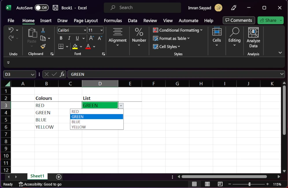
First, create a list of colors that you want to include in the drop-down list. You can do this by typing the colors into a range of cells, or by using the COLOR function to generate a list of colors based on their RGB values. the colour name list may be such as,

• RED
• GREEN
• BLUE
• YELLOW

Step 2: Create a dropdown list with data validation

Next, select the cell or cells where you want to create the drop-down list, and then go to the Data tab and click on the Data Validation button.

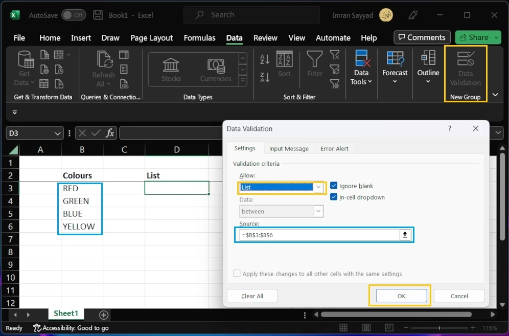
In the Data Validation dialog box, select the List option under Allow, and then enter the cell range for your list of colors in the Source field or give reference to the cells containing color names. Here =$B$3:$B$6

Click OK to apply the data validation. You should now see a drop-down arrow next to the cell, which you can use to select a color from the list.

Step 3: Set fill color from conditional formatting

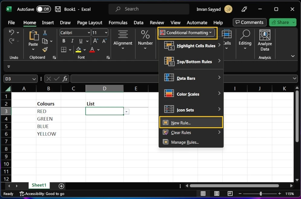
Now create a new rule for the list cell from the conditional formatting option. Set the rule type: “Format only cells that contain”

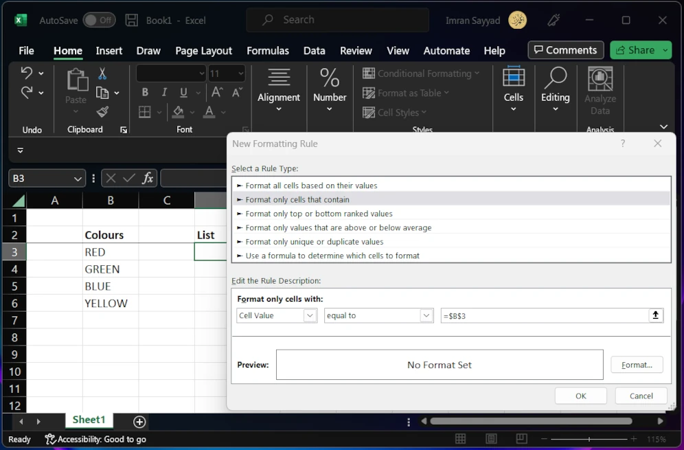
As shown in the above screenshot, create a rule for each color as Cell Value->equals to-> =cell ref (here =$B$3 for RED color). Then click on “Format” to set color fill for that rule.

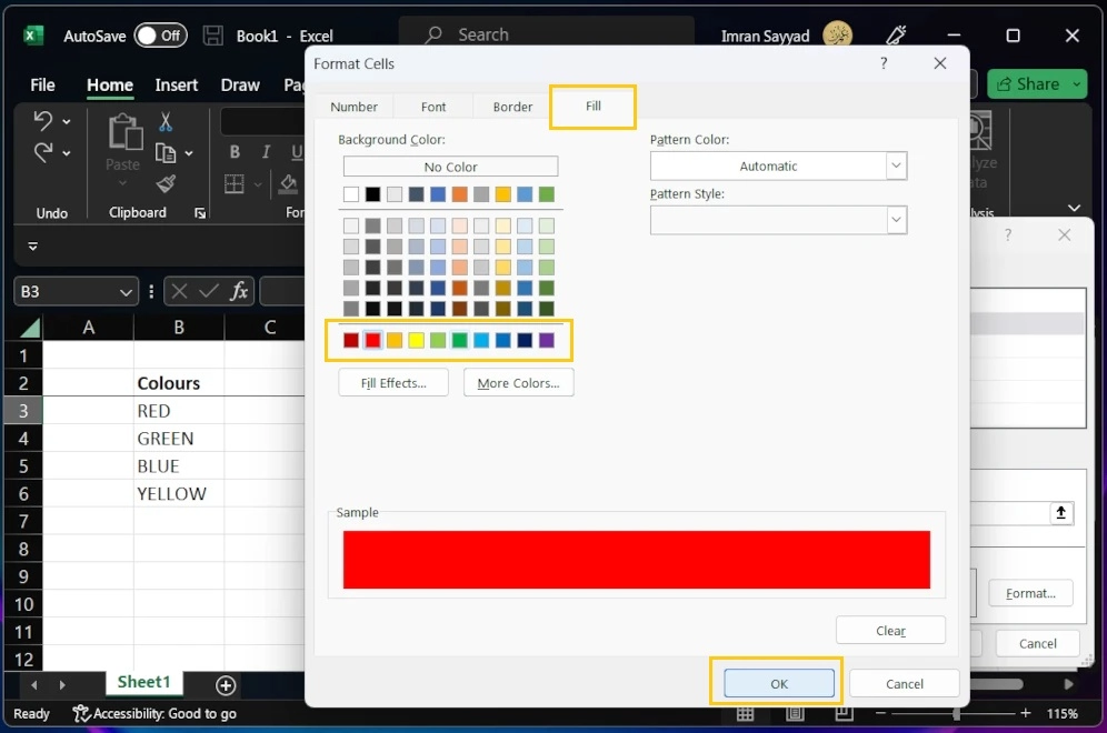
As shown in the above screenshot, set the required fill color (here RED).
Then click on OK.

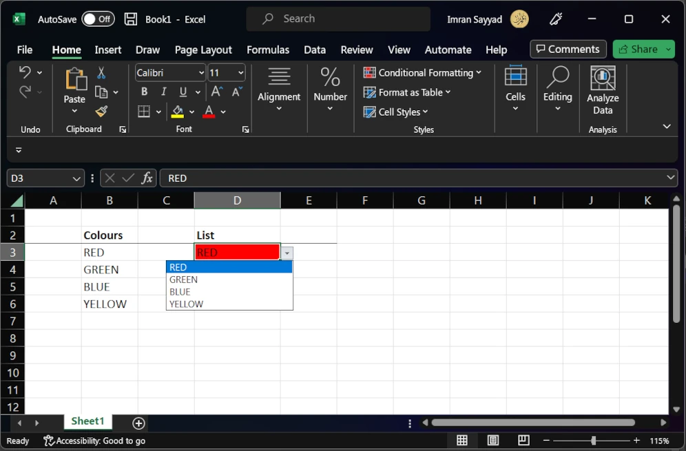
Repeat step 3 for each color.

If you want to display the colors in the drop-down list as actual colors, rather than just the names of the colors, you can use the CONVERT function to convert the RGB values to a color code that Excel can recognize.

For example, you can use the formula =CONVERT(B3, "RGB", "HTML") to convert the RGB value in cell A1 to a color code. You can then use this formula in the cells next to your list of colors to create a color-coded drop-down list.

Here are a few more tips for creating a drop-down list with colors in Excel:

1. Use the COLOR function to generate a list of colors: The COLOR function allows you to generate a color based on its RGB values. You can use this function to create a list of colors by entering a range of RGB values in the formula. For example, you can use the formula =COLOR(ROW(A1:A10), COLUMN(A1:A10), 0) to generate a range of colors from red to green.
2. Use named ranges: If you are creating a long list of colors, it can be easier to manage the list if you use named ranges. To create a named range, select the cells you want to include in the range, and then go to the Formulas tab and click on the Define Name button.
3. Use the Conditional Formatting feature: If you want to display the colors in the drop-down list as actual colors, you can use the Conditional Formatting feature to apply a color to the cells based on their values. To do this, select the cells where you want to apply the formatting, and then go to the Home tab and click on the Conditional Formatting button. In the Conditional Formatting dialog box, select the Color Scale option, and then choose a color scale to apply to the cells.
4. Use the REPT function: The REPT function allows you to repeat a character or string a specified number of times. You can use this function to create a series of color swatches in a column, and then use the INDEX and MATCH functions to return the corresponding color name from your list of colors.